In this article, we show how we analyzed the Citi Bike trips dataset{" "} and built a model to predict ridership based on seasonality{" "} and weather.

Introduction

Citi Bike opened in New York City in 2013 and has since grown in ridership, bikes, and bike dock stations. Predicting demand for bikes is important for Motivate, Citi Bike’s parent company, in order to both reduce operating costs and increase ridership. Costs are incurred by having under-utilized bikes on the streets, by wear-and-tear on bikes due to exposure to the elements, or other forms of damage, so it is necessary to warehouse bikes if they are not serving riders. However, having too few available bikes leads to a poor customer experience and eventual loss of revenue due to dissatisfied customers, so a balance must be struck.

In this capstone project, we first tried to understand what drives demand for bikes—time, weather, etc. Then, we created a predictive model based on our data analysis. Finally, we compared our model against the actual number of trips to evaluate its usefulness.

Analyzing the data

We focused our exploratory data analysis on

• Rider demographics
• Citi Bike’s growth
• Demand during the pandemic
• Time (and Seasonality)
• Temperature and Weather Conditions

and determined predictors for our time-series model from that analysis.

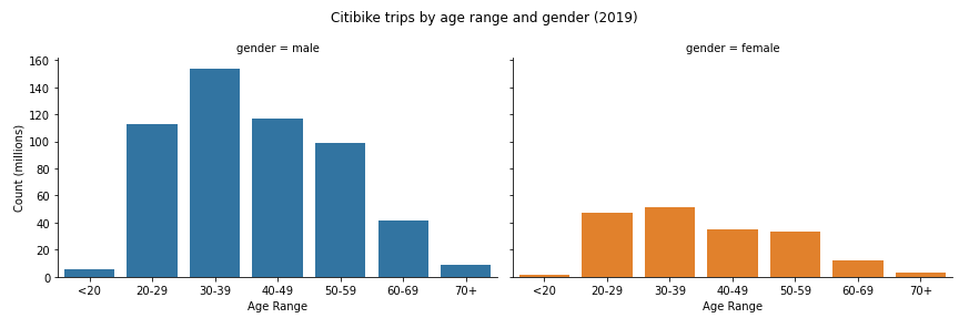
Demographics

By age, most riders are between 20 and 40 years and are mostly male. Citi Bike has two classes of riders—annual subscribers and single-ride or day pass purchasers.

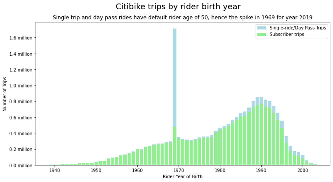
We see a spike in trips by a rider’s year of birth for the year 1969. This is due to Citi Bike setting a default age of 50 years for riders purchasing one-off trips or passes.

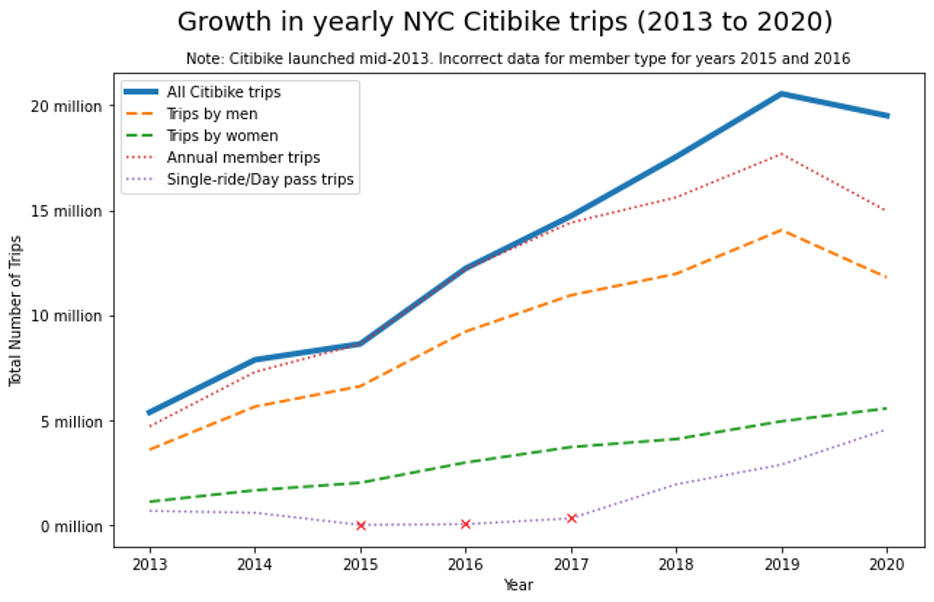
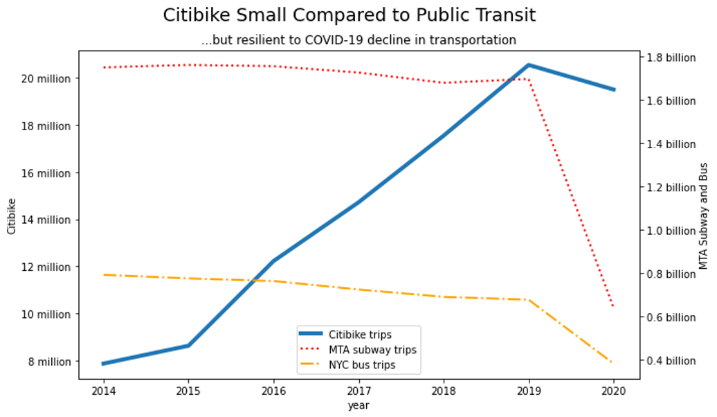
Growth and Resilience of Citi Bike

As the number of Citi Bike trips grows, operational efficiency is more important to company finances. In addition, there is need for accurately predicting demand and rebalancing stations effectively

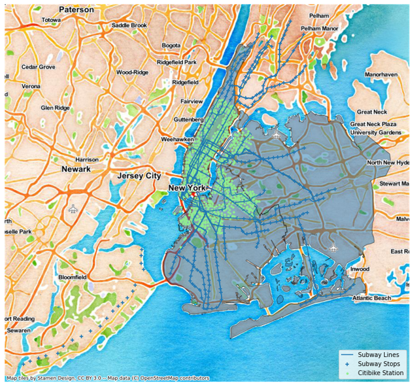
Bike stations appear to expand along subway lines…potential for further expansion into Brooklyn, the Bronx, or Queens?

While Citi Bike is not used as much as mass transit in NYC, it offered a way for city residents to move from A to B during the pandemic that wasn’t in an enclosed space…perhaps this is why it didn’t see as sharp a drop in demand compared to the NYC subway or buses

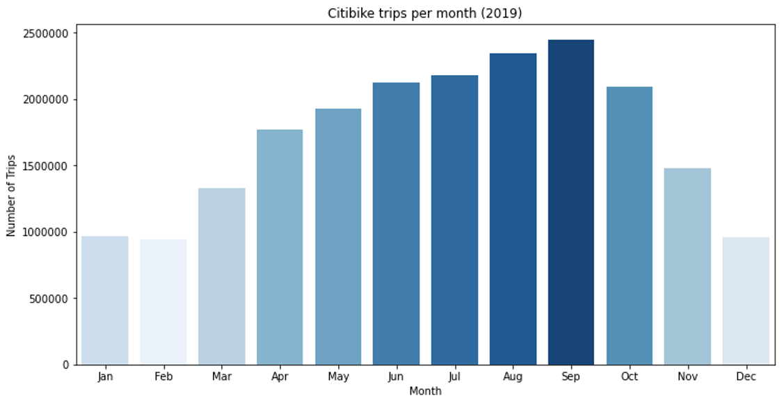
Temporal Analysis

We see increased usage in the summer as one might expect, but not all summer days prove to have high counts.

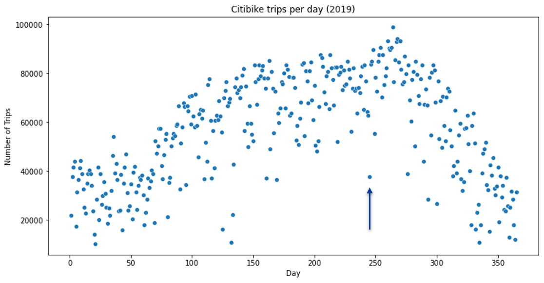
Labor Day, 2019 shows reduced demand…and weather might also play an effect. We examine that later.

Surprisingly, weekends, especially Sunday, seem to have lower trip counts on average than weekday. Sunday truly is the day of rest.

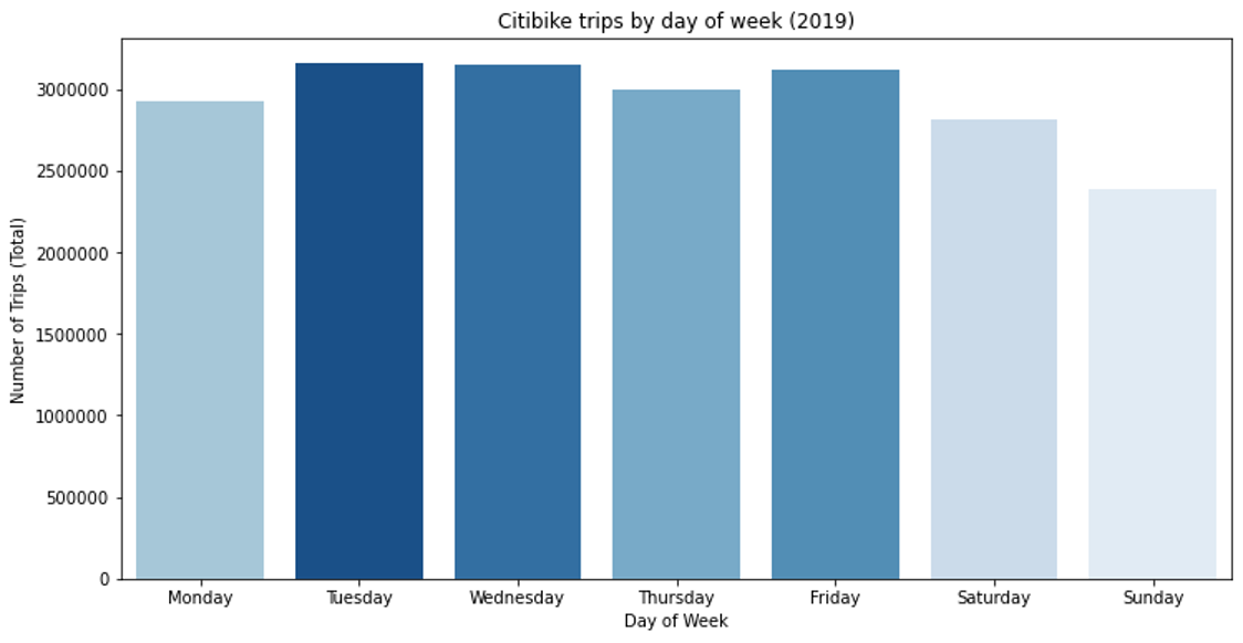
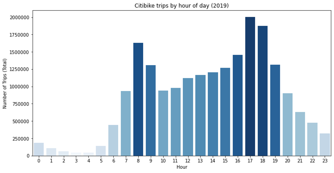
It looks like commuters make up a bulk of trips given the high trip counts around 8am and 5pm. This also explains the reduced number of trips on weekends.

Weather

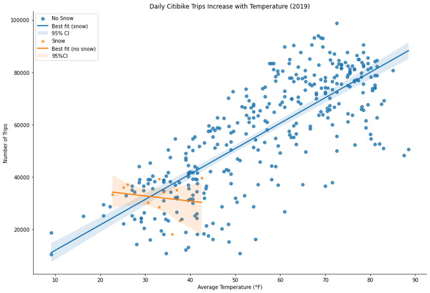
We began by looking at daily average temperature and found that trip demand is linearly correlated with it. We can use this as a model predictor!

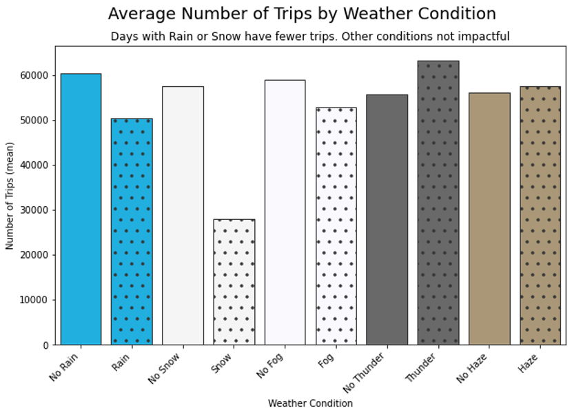
We wanted to investigate whether weather conditions might have an effect on number of trips…however, we only saw a decrease for days with precipitation (rain/snow).

There were few days with fog, thunder, or haze and the effect (oddly, positive for thunder and haze) is minor in comparison to rain and snow.

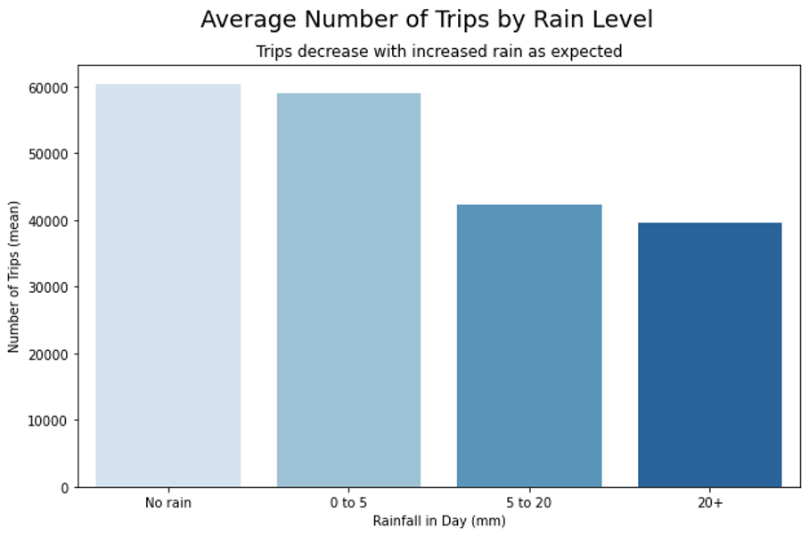
Digging deeper, we wanted to see if the amount of rain mattered…and it does! (As one expects)

Based on this analysis, we decided to create a model incorporating time, average temperature, and amount of precipitation in order to predict the number of trips.

Trip Demand Prediction Models

We attempted two models, the first of our models is the traditional SARIMA model, the second was a Long Short-Term Memory Recurrent Neural Network (LSTM-RNN). In this, we further distinguish the models by the time resolution, and whether or not the model was including weather data (i.e. had multidimensional inputs). Notably absent from our treatment is a vectorized SARIMA model or SVARIMA; however, this was due to time considerations and the fact that LSTM models on average demonstrate far better performance on multidimensional time series than traditional models and approaches.

The population data is found in in the seconds resolution; however, at this resolution, observations are not continuously present and we have long gaps for many seconds of the year with zero ridership. We take a look at the hourly ridership data from 2019; whatever model we create for one year we can easily generalize to multiple years.

As a preliminary assessment of the data, we look at the ridership over the year along different timescales—in doing so we can begin to understand trends and seasonality relationships within the day. Changing the scale of our data, as we will see, is akin to passing the “wave” of our time series through a low-pass filter, giving us lower frequency relationships. Therefore, if there is high seasonality at low timescale, this will be erased as we increase our timescale and aggregate over larger steps.

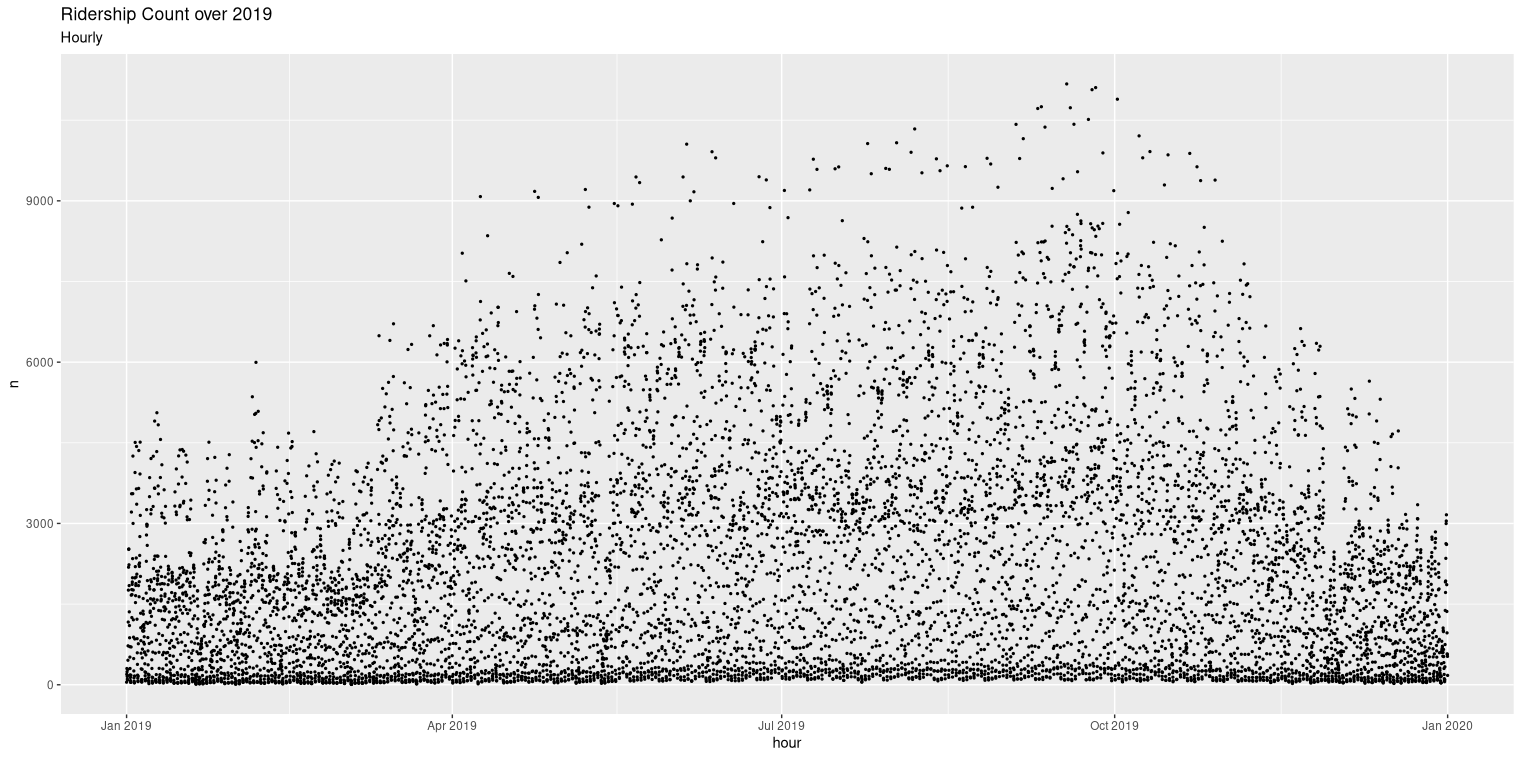
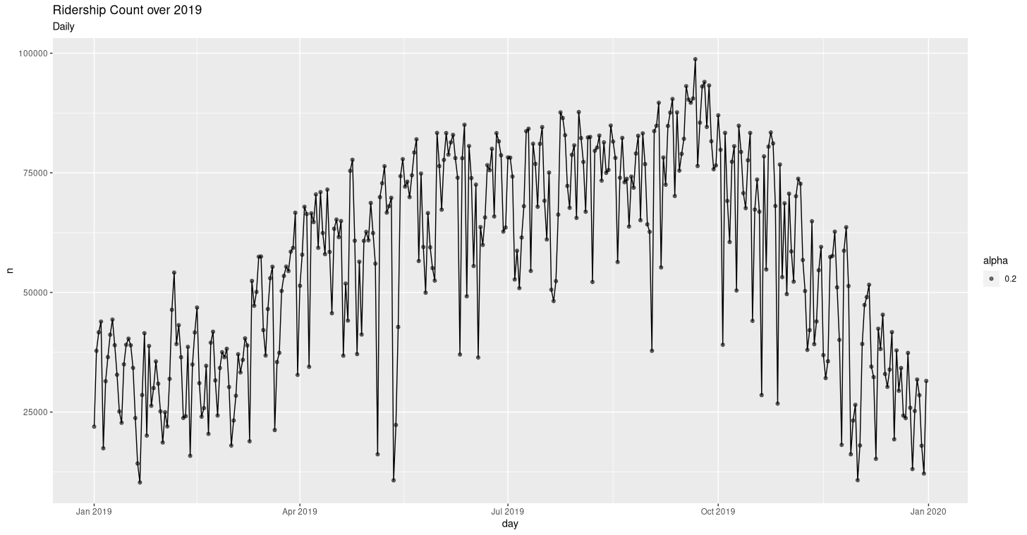
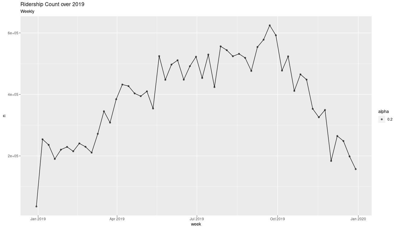
We can see from the above graphs that weekly resolution is far too sparse to capture meaningful relationships. Therefore, we would like to build models that predict at the Hourly timescale if we can, and if not, then use the Daily timescale

At the sub hourly timescale, the data became too unwieldy and noisy for a years worth, let alone for the many years of data Citi Bike has available. However in future extensions of this project we would like to take a second level resolution for one week for one station and predict the ridership at that level.

Our models were thus:

1. Daily SARIMA, which did not converge to parameters.
2. Daily LSTM with weather, which had reduced RMS error.
3. Hourly LSTM without weather, which had great success.

We compared these models by producing the Daily and Hourly RMSE and comparing them to find the RMSE minimizing model.

Based on our results, we would believe that an hourly LSTM for a specific station, with weather, will be the best model, and this is the model we will investigate for further research. However, we found that including the weather data, while good at predicting trends in average ridership, is not as good at predicting the noise, which is only captured at the hourly level.

Seasonal-differencing autoregressive integrated moving average (SARIMA)

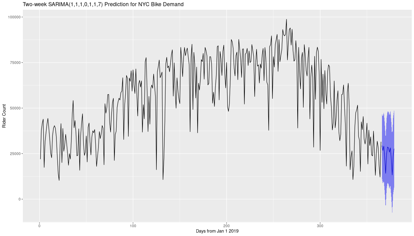
SARIMA(1 1 1 0 1 1 7) AIC= 7761.436  SSE= 53381920877  p-VALUE= 0.821252

Above is the two week prediction for the two week ridership given the entire years worth of data. The line is our median prediction and the section on the right is the 95% confidence interval. We see that our prediction model has a SSE of 53381920877, giving us a RMSE of 231,045 ^bikes^⁄day! This is our number to beat.

Long short-term memory recurrent neural network (LSTM)

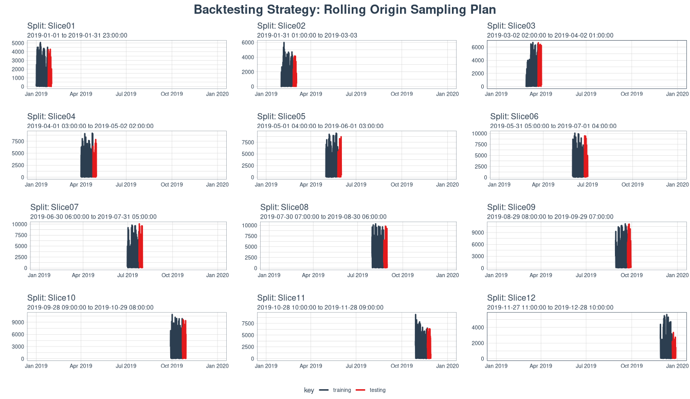
1. Daily LSTM (with Weather)—Backtesting Strategy

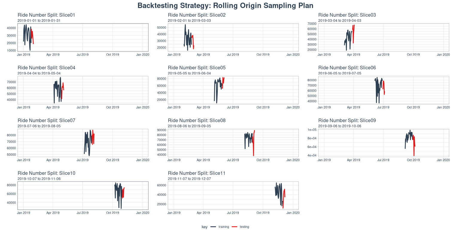
Above we see the backtesting split and the train test split for each backtest slice. We can see the progression of each of the splits through the year. Zooming into each split, we have:

2. Daily LSTM (with Weather)—Predictions

First, let us take a look at how the Temperature and Average Precipitation data influences the ridership number. Below we see the Ridership, Average Temperature, and Average Rainfall over the entire year of 2019.

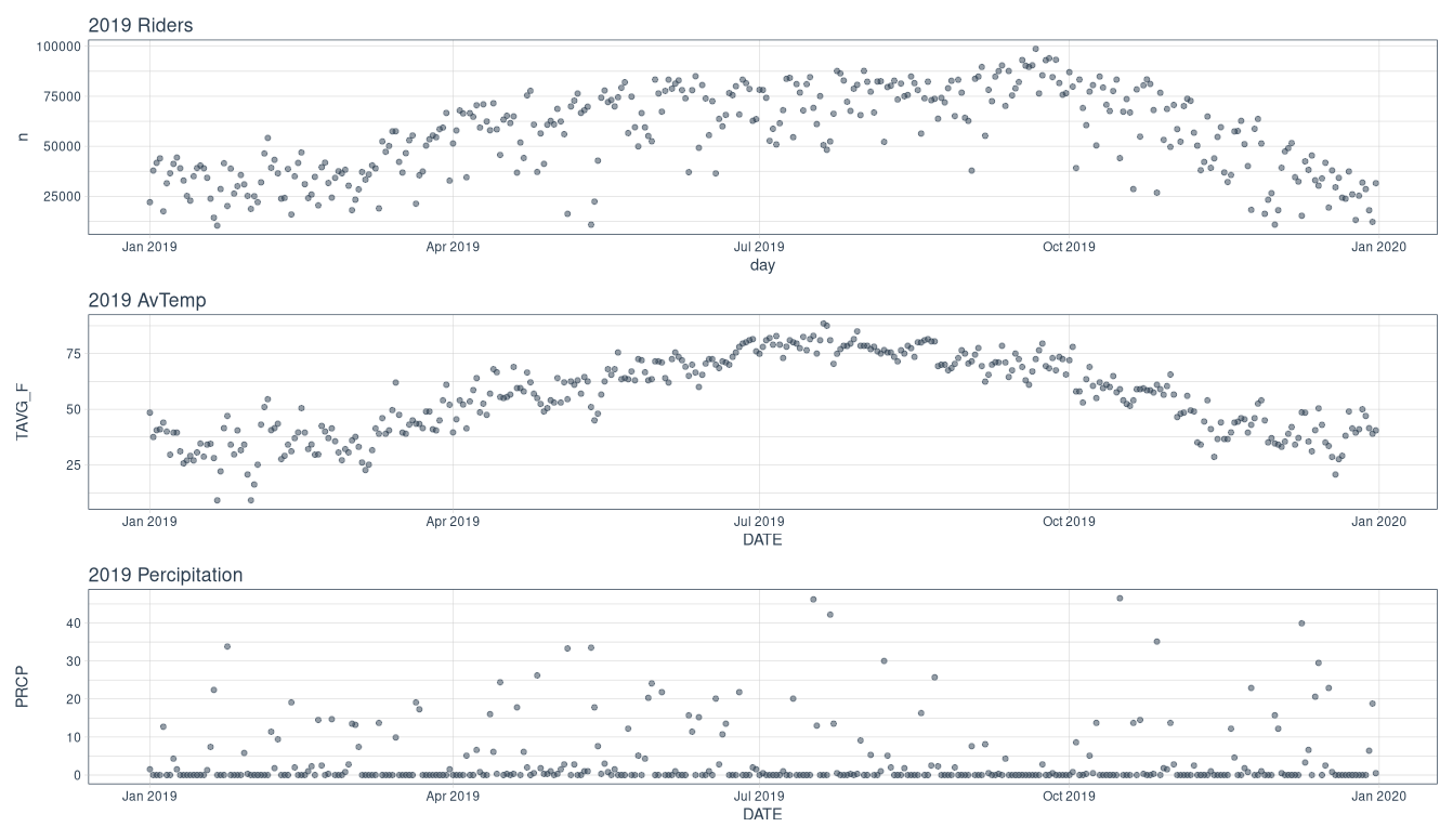
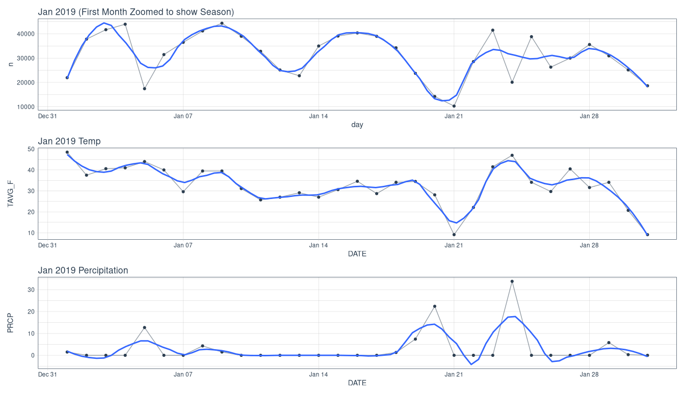
Zooming into the January, we can see that there is clear monthly, and weekly seasonality. Furthermore, there seems to be a direct correlation between average temperature and ridership, and an inverse correlation between precipitation and ridership.

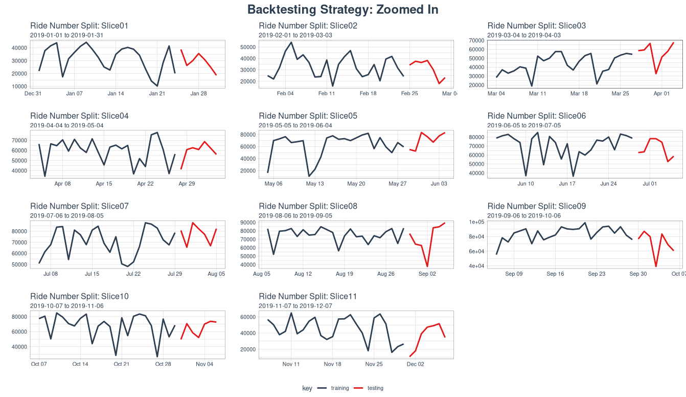
We can see the predictions over each of the backtesting slices to get an idea of how our model looks like after training, and without early-stopping to correct for overfitting. Below, we see each slice with their prediction, and each RMSE value.

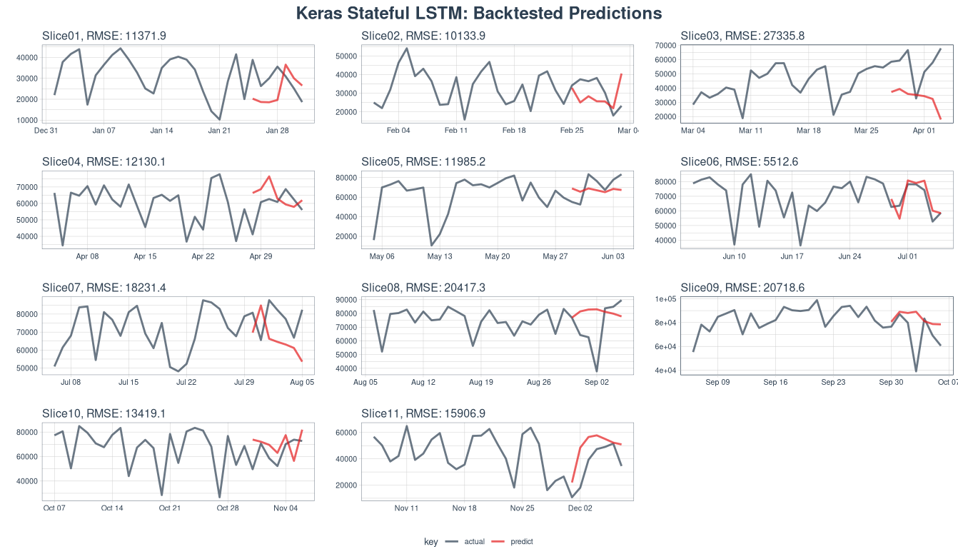
While these predictions don’t look particularly impressive against our data, keep in mind that a lot of the jaggedness of the data comes from the fact that ridership can jump drastically between days due to a number of factors.

The mean RMSE was 15197 ^bikes^⁄day with standard deviation of ±6097 ^bikes^⁄day.

Thus, moving to an LSTM model with weather greatly improved our daily RMSE, and this is a significant enough improvement to warrant exploring the LSTM approach further.

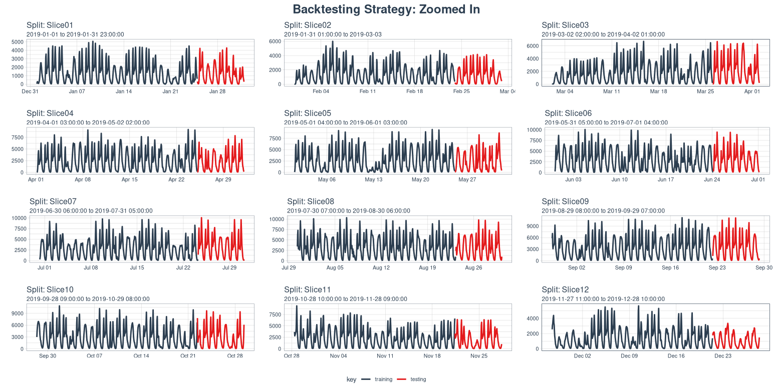
3. Hourly LSTM (without Weather)—Backtesting Strategy and Predictions

Going down to the hourly timescale, without including the weather data, we have already seen that the full years worth of data is extremely noisy. Looking at our backtesting strategy, we can see that reflected. Zooming into each month, we can see that there is a sub-daily seasonality to the data that we have been unable to capture.

Fitting an LSTM model to these, we reach the following backtesting predictions.

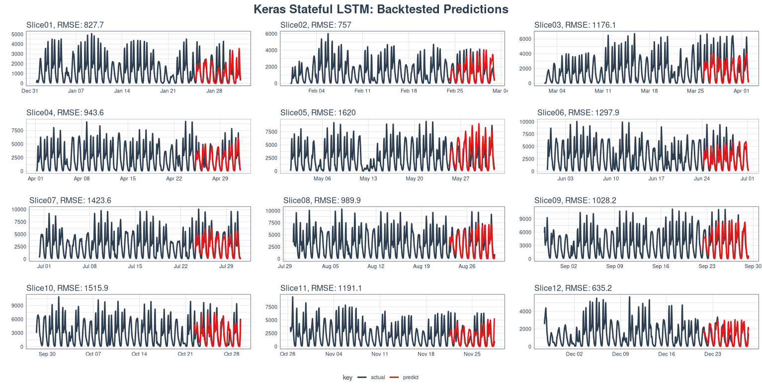
We have an mean daily RMSE of 26,812 ^bikes^⁄day. We can see that these models look much more predictive of the oscillations in the data; however, we also calculated the daily and hourly errors naively and the prediction resolution we get is much stronger in the hourly timescale—hence, the hourly model is better.

Conclusion

Our exploratory data analysis informed our model feature selection and we attempted two time-series models (SARIMA and LSTM) to predict trip demand on both an hourly and daily basis. We found that hourly models were better overall. Further improvements to the model would be in reducing the root mean square error in predictions and, perhaps, incorporating additional predictors.

Those seeking to improve upon our approach might like to build an LSTM model for each bike dock station on an hourly timescale, while accounting for weather. Predicting by bike station while filtering for the top stations by number of trips might be more useful for Citi Bike’s operations team.

If you found this article interesting, please reach out! You can also read our follow-up analysis on Citi Bike’s rebalancing operations.